For our first joint blog post we decided to look at this week’s #TidyTuesday dataset. Tidy Tuesday is a weekly data project aimed at the R for Data Science community. Every week a raw dataset is posted so that users can apply their R skills, get feedbak, explore other’s work, and connect with the greater #RStats community.
This week’s data is about Board Games! The data comes from the Board Game Geek database.
The first step is to download the dataset from the TidyTuesday Repository.
board_games <- readr::read_csv("https://raw.githubusercontent.com/rfordatascience/tidytuesday/master/data/2019/2019-03-12/board_games.csv")Building a Linear Model
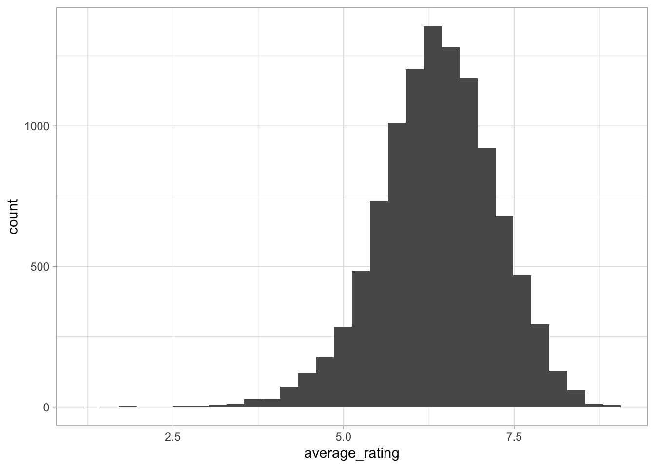
For this dataset we want to see if we can build a model to predict how sucessful a game’s rating might be. We begin by looking at the distribution of the average rating variable.
board_games %>%
  ggplot(aes(average_rating))+
  geom_histogram()
Average rating has an almost normal distribution which is good because it means we can apply a linear model to predict rating.
reg1<-lm((average_rating) ~ log2(max_players + 1) +log2(max_playtime+1) + year_published, data = board_games)
summary(reg1)
##
## Call:
## lm(formula = (average_rating) ~ log2(max_players + 1) + log2(max_playtime +
## 1) + year_published, data = board_games)
##
## Residuals:
## Min 1Q Median 3Q Max
## -4.9862 -0.4437 0.0230 0.4800 2.8934
##
## Coefficients:
## Estimate Std. Error t value Pr(>|t|)
## (Intercept) -4.670e+01 1.214e+00 -38.46 <2e-16 ***
## log2(max_players + 1) -1.951e-01 1.031e-02 -18.92 <2e-16 ***
## log2(max_playtime + 1) 1.664e-01 4.538e-03 36.68 <2e-16 ***
## year_published 2.627e-02 6.049e-04 43.44 <2e-16 ***
## ---
## Signif. codes: 0 '***' 0.001 '**' 0.01 '*' 0.05 '.' 0.1 ' ' 1
##
## Residual standard error: 0.748 on 10528 degrees of freedom
## Multiple R-squared: 0.2266, Adjusted R-squared: 0.2264
## F-statistic: 1028 on 3 and 10528 DF, p-value: < 2.2e-16In this model we infer how well the maximum number of players, the maximum of amount of playtime, and the year that the game was published predicts the rating. Everytime you double maximum number of players expect average rating to go down by 0.195 on average. Doubling max playtime will leads to a 0.166 increase in the average rating. \(R^2\) value shows that the model explains 22.6% of the data. And all the varibales are statstically significant.
Tidyverse
We noticed that the Category variable contains many values seperated by comma. We decided to use the tidyverse “separate_rows” function to seperate this variable into multiple rows, this will make it easier to analyze.
categorical_variables<- board_games %>%
  select(game_id, category) %>%
  gather(type, value, -game_id) %>%
  filter(!is.na(value)) %>%
  separate_rows(value, sep = ",")
GGplot Visualization
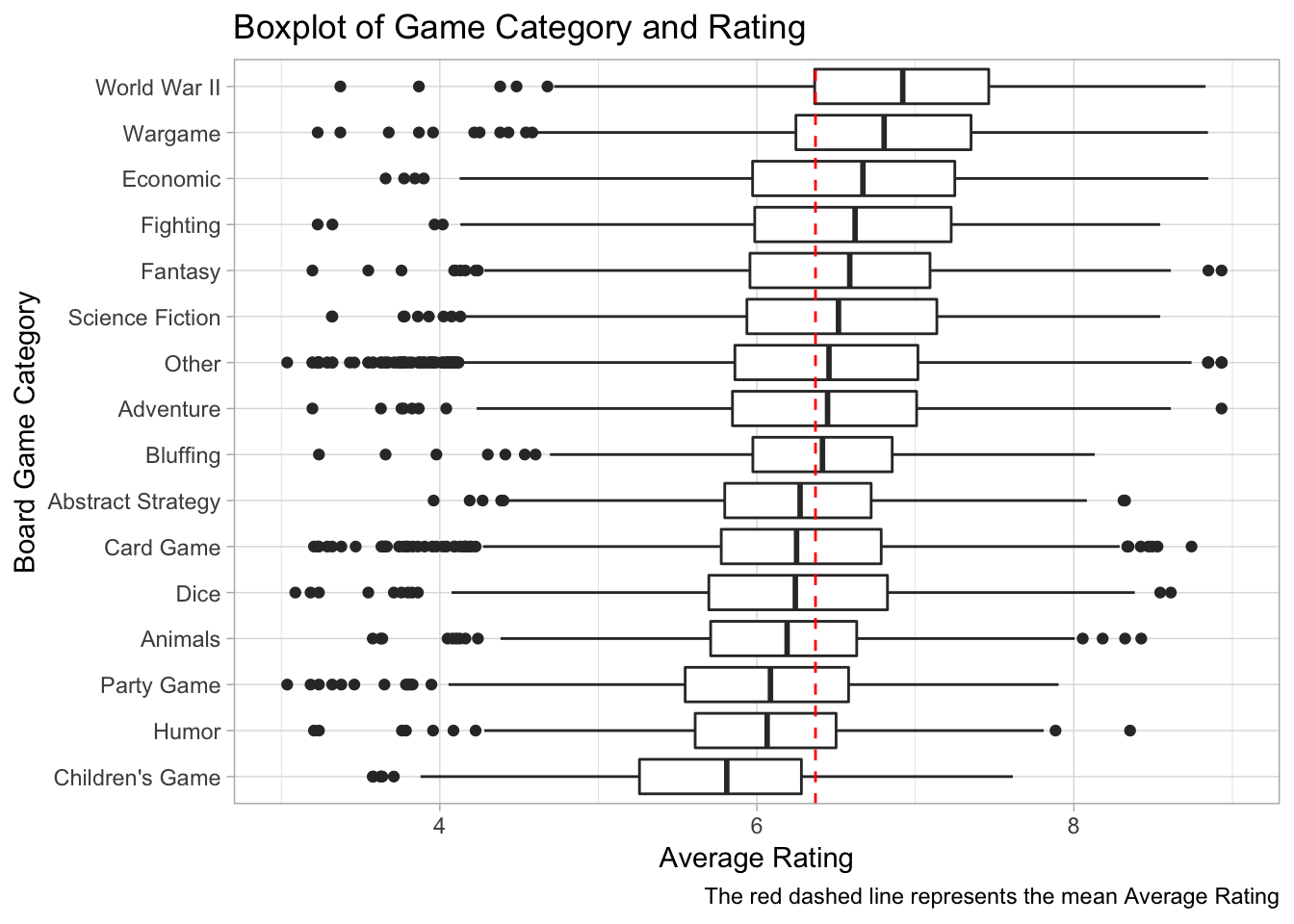
For this visualization we want to make a boxplot of average rating by category. This will help us understand which categories correlate with higher ratings.
board_games %>%
  inner_join(categorical_variables, by = c("game_id")) %>%
  filter(type == "category") %>%
  mutate(value = fct_lump(value, 15),
         value = fct_reorder(value, average_rating)) %>%
  ggplot(aes(value, average_rating)) +
  geom_boxplot()+
  coord_flip()+
   ylim(3,9) +
  geom_hline(yintercept=6.37, linetype="dashed", color = "red")+ #Adding a vertical line at the mean
  labs(y="Average Rating", x = "Board Game Category", title = "Boxplot of Game Category and Rating", caption= "The red dashed line represents the mean Average Rating")